
Desktop Survival Guide
by Graham Williams
|
|
DATA MINING
Desktop Survival Guide by Graham Williams |
|
|||
Lung |


|
> l.survreg <- survreg(l.Surv ~ age, data=lung) > summary(l.survreg) |
Call:
survreg(formula = l.Surv ~ age, data = lung)
              Value Std. Error     z        p
(Intercept)  6.8871     0.4466 15.42 1.20e-53
age         -0.0136     0.0070 -1.94 5.19e-02
Log(scale)  -0.2761     0.0624 -4.43 9.61e-06

Scale= 0.759

Weibull distribution
Loglik(model)= -1151.9   Loglik(intercept only)= -1153.9
	Chisq= 3.91 on 1 degrees of freedom, p= 0.048
Number of Newton-Raphson Iterations: 5
n= 228
|
> l.pred <- predict(l.survreg, lung)
> l.pred.q <- predict(l.survreg, lung, type="quantile")
> result <- cbind(data.frame(lung$time, l.pred), l.pred.q)
> names(result) <- c("Actual", "Predicted", "Lower", "Upper")
> head(result)
|
Actual Predicted Lower Upper 1 306 357.8476 64.88637 673.7982 2 455 388.2918 70.40663 731.1220 3 1010 457.1705 82.89600 860.8152 4 210 450.9914 81.77557 849.1803 5 883 432.9505 78.50432 815.2108 6 1022 357.8476 64.88637 673.7982 |
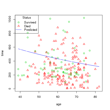
Plot age versus time, and status, then draw line byt age with the predicted survival time:
> ord <-order(lung$age)
> age_ord <- lung$age[ord]
> pred_ord <- l.pred[ord]
> with(lung, plot(age, time, pch=status, col=4-status))
> lines(age_ord, pred_ord, col=4)
> legend("topleft", title="Status", c("Survived", "Died", "Predicted"),
         pch=c(1, 2, -1), lty=c(0,0,1), col=c(3,2,4))
|
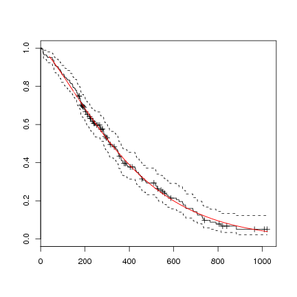
You can not plot the survreg directly, but could do the following, using the coefficients from the regression formula, which will also give a hint in interpreting the formula:
> l.survreg.weibull <- survreg(l.Surv ~ 1, data=lung, dist='weibull')
> plot(survfit(l.Surv~1, data=lung))
> curve(exp(-(exp(-l.survreg.weibull$coef[1]) * x)^(1/l.survreg.weibull$scale)),
        col="red", add=TRUE)
|
Another example this time we fit a parametric survival model with a Weibull distribution for time to death fitting a different shape parameter for each gender, by using a strata term.
> l.survreg <- survreg(l.Surv ~ ph.ecog + age + strata(sex), lung) > print(l.survreg) |
Call:
survreg(formula = l.Surv ~ ph.ecog + age + strata(sex), data = lung)

Coefficients:
(Intercept)     ph.ecog         age
 6.73234505 -0.32443043 -0.00580889

Scale:
    sex=1     sex=2
0.7834211 0.6547830

Loglik(model)= -1137.3   Loglik(intercept only)= -1146.2
	Chisq= 17.8 on 2 degrees of freedom, p= 0.00014
n=227 (1 observation deleted due to missingness)
|
> summary(l.survreg) |
Call:
survreg(formula = l.Surv ~ ph.ecog + age + strata(sex), data = lung)
               Value Std. Error      z        p
(Intercept)  6.73235    0.42396 15.880 8.75e-57
ph.ecog     -0.32443    0.08649 -3.751 1.76e-04
age         -0.00581    0.00693 -0.838 4.02e-01
sex=1       -0.24408    0.07920 -3.082 2.06e-03
sex=2       -0.42345    0.10669 -3.969 7.22e-05

Scale:
sex=1 sex=2
0.783 0.655

Weibull distribution
Loglik(model)= -1137.3   Loglik(intercept only)= -1146.2
	Chisq= 17.8 on 2 degrees of freedom, p= 0.00014
Number of Newton-Raphson Iterations: 5
n=227 (1 observation deleted due to missingness)
|