Desktop Survival Guide
by Graham Williams
|
|
DATA MINING
Desktop Survival Guide by Graham Williams |
|
|||
Predictive Analytics |


|
Using our data to discover new knowledge that we can deploy to better improve our business processes is the key to data mining. We will often want to predict something about new observations based on our historic data. The tasks of classification and regression are at the heart of what we often think of as data mining. Indeed, we call much of what we do in data mining Predictive Analytics. From a machine learning perspective this is referred to as supervised learning.
Traditional data mining focuses on algorithms developed for Artificial Intelligence and Machine Learning. This research has generally focused on building so called classification models. Such models are used to classify new observations into different classes. Often we will be presented with just two classes, but it could be more. A new observation might be a new day, and we want to classify it into whether there might be rain on that day, or not.
Statisticians have traditionally focused on the alternative view the task as one of regression. The aim here is to build a mathematical formula that aims to capture the relationship between a collection of input variables and a numeric output variable. This formula can then be applied to new observations to predict a numeric outcome. The new observation might be a new day, and we want to predict the amount of for that day.
Interestingly, regression comes from the word ``regress,'' which means to move backwards. It was used by () in the context of techniques for regressing (i.e., moving from) observations to the average. The early research included investigations which separated people into different classes based on their characteristics. The regression came from modelling the heights of related people (, ).
The machine learning and statistical contributions to data mining has lead to different perspectives on the same tasks. Together they complement each other and provide important tools for the data miner's toolbox.
As well as building a model so that we can apply the model to new data (the predictions), we look to the structure of the model itself to provide insights. In particular, we can learn much about the relationships between the input variables and the output variable from studying our models. Sometimes these observations themselves deliver benefit from the data mining project.
This chapter focuses on the classification and regression tasks--collectively referred to as building predictive models. We will introduce the common data mining algorithms for predictive modelling. Each is presented in the context of the framework for understanding models presented in Section 1.5. There we identified the three components of a modelling algorithm: a knowledge representation language, a quality measure, and heuristics for searching for the better sentences in the language.
For each algorithm we describe its usage, provide illustrative examples and specify psuedo-code for the algorithm, providing insights into how the algorithm works and some detail allowing a programmer to implement the algorithm. Pointers to further information lead the interested reader to the literature covering the algorithm in much more detail.
The algorithms we present will generally be in the context of two class classification task. The aim of such tasks is to distinguish between two classes of observations. Such problems abound. The two classes might, for example, identify whether or not it is predicted to rain tomorrow, distinguish high risk and low risk insurance clients, productive and unproductive taxation audits, responsive and non-responsive customers, successful and unsuccessful security breaches, and so on.
In this chapter we will cover the following algorithms for classification and regression: Decision Trees, Boosted Decision Trees, Random Forests, Support Vector Machines, Neural Networks, and Logistic Regression.
Once again we will demonstrate the tasks using Rattle together with a guide to the underlying R code. Rattle presents a basic collection of tuning parameters through its interface for building models. Rattle presents good default values for various options to allow the user to more simply build a model with little tuning. This may not always be the right approach, but is certainly a good place to start.
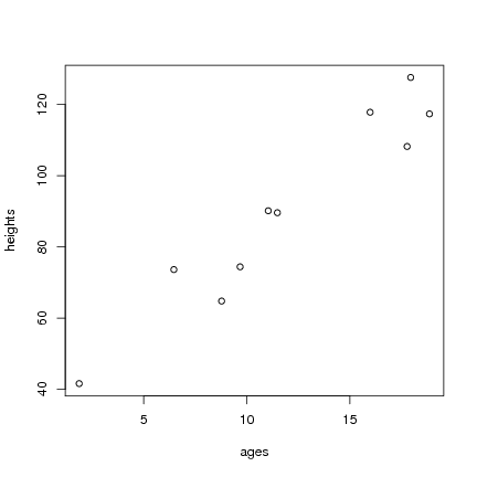
Let's have a look at the simplest of problems. Suppose we want to model one variable (e.g., a person's height) in terms of another variable (e.g., a person's age).
We can create a collection of people's ages and heights, using some totally random data. First we set the seed, using set.seed, so that the random data is the same each time we run this example. We then generate random ages and random heights, but the random heights are based on the age.
> set.seed(123) # To ensure repeatability. > ages <- runif(10, 1, 20) # Random ages between 1 and 20 > heights <- 30 + rnorm(10, 1, as.integer(ages)) + ages*5 > plot(ages, heights) |
We can now build a model (in fact, a linear interpolation) that approximates this data using R's approxfun function:
> my.model <- approxfun(ages, heights) > my.model(15) |
[1] 111.6762 |
> plot(ages, heights) > plot(my.model, add=TRUE, col=2, ylim=c(20,200), xlim=c(1,20)) |
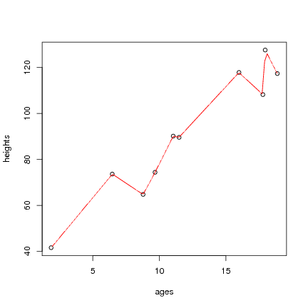
From the resulting plot we can see it is only an approximate model and indeed, not a very good model. The data is pretty deficient, and we also know that generally height does not decrease for any age group in this range. It illustrates the modelling task though.
> my.spline <- splinefun(ages, heights) |