Archive for year: 2016

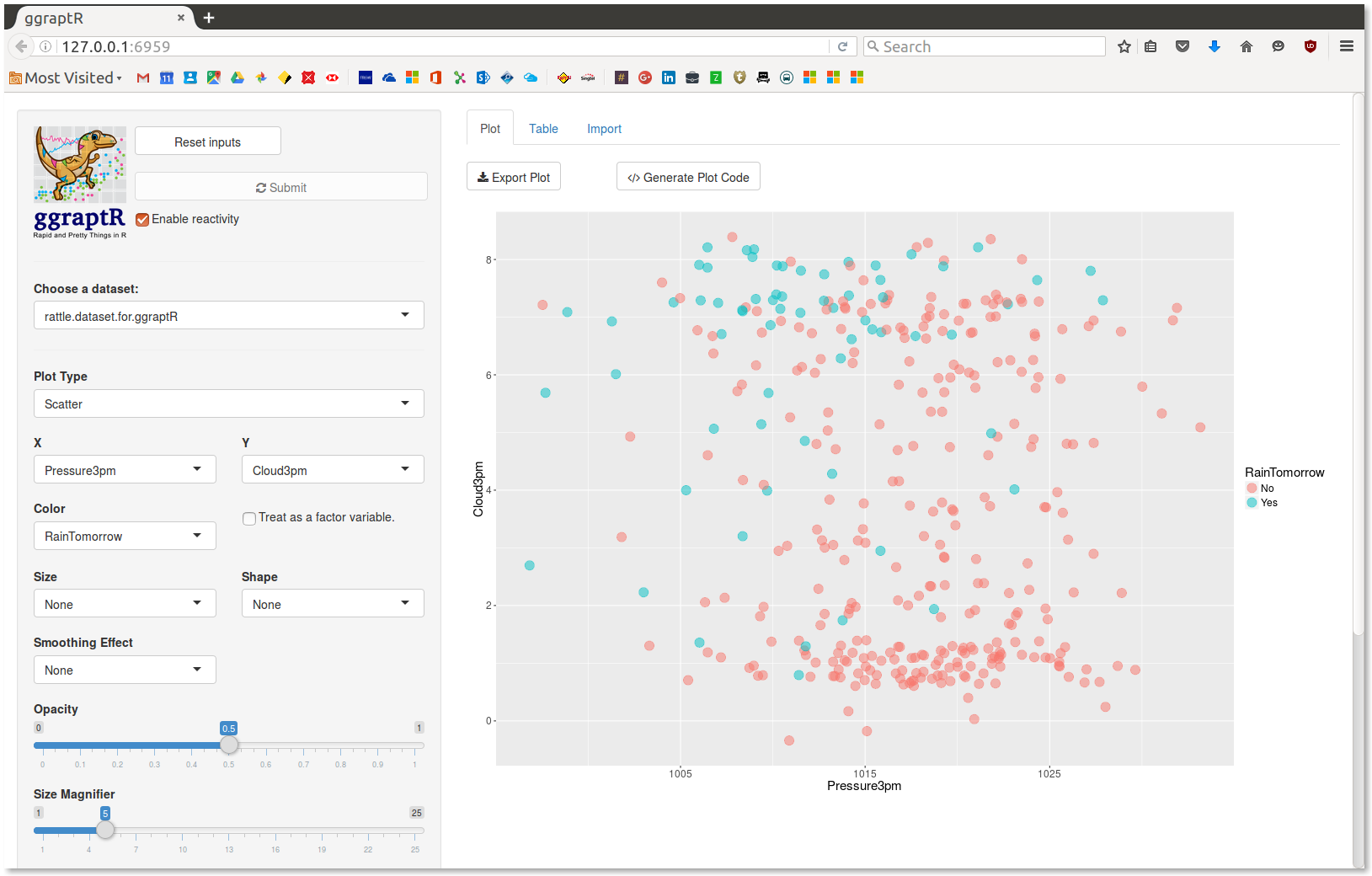
Data Scientists have access to a grammar for preparing data (Hadley Wickham’s tidyr package in R), a grammar for data wrangling (dplyr), and a grammar for graphics (ggplot2).

At an R event hosted by CSIRO in Canberra in 2011 Hadley  noted that we are missing a grammar for machine learning. At the time I doodled some ideas but never developed. I repeat those doodles here. The idea’s are really just that – ideas as a starting point. Experimental code is implemented in the graml package for R which is refining the concepts first explored in the experimental containers package.

A grammar of machine learning can follow the ggplot2 concept of building layer upon layer to define the final model that we build. I like this concept rather than the concept of a data flow for model building. With a data flow a dataset is piped (in R using magrittr’s %>% operator) from one data wrangling step to the next data wrangling step. Hadley’s tidyr and dplyr do this really well.

The concept of a grammar of machine learning begins with recognising that we want to train a model:

train(ds, form(target ~ .))

Simply we want to train a model using some dataset ds where one of the columns of the dataset is named target and we expect to model this variable based on the other variables within the dataset (signified by the ~ .).

Generally in machine learning and statistical model building we split our dataset into a training dataset, a validation dataset, and a testing dataset. Some use only two datasets. Let’s add this in as the next “layer” for our model build.

train(ds, form(target ~ .)) +
  dataPartition(0.7, 0.3)

That is, we ask for 70% of the data randomly sampled to train the model.

We will have already performed our data preparation steps and let’s say that we know in ds the target variable has only two distinct values, yes and no. Thus a binary classification model is called for.

In R we have a tremendous variety of model building algorithms that support binary classification. My favourite has been randomForest so let’s add in our request to train a model using randomForest().

train(ds, formula(target ~ .)) +
  dataPartition(0.7, 0.3) +
  model(randomForest)

Now we might want to do a parameter sweep over the mtry parameter to the randomForest() function which is the number of variables to randomly sample as we build each decision tree.

train(ds, formula(target ~ .)) +
  dataPartition(0.7, 0.3) +
  model(randomForest) +
  tuneSweep(mtry=seq(5, nvars, 1))

Finally to report on the evaluation of the model using the area under the curve (AUC).

train(ds, formula(target ~ .)) +
  dataPartition(0.7, 0.3) +
  model(randomForest) +
  tuneSweep(mtry=seq(5, nvars, 1)) +
  evaluate_auc()

The object returned is a trained model incorporating the additional information requested. Other operations can be performed on this model object, including its deployment into a production system!

We can provide parameters as a lightweight layer above other model building packages with no or minimal effort required to move to a new model builder.

  model(randomForest::randomForest, 
        ntree=100, 
        mtry=4, 
        importance=TRUE,
        replace=FALSE, 
        na.action=randomForest::na.roughfix)

(Image from http://grammar.ccc.commnet.edu/grammar/)

Graham @ Microsoft